class: center, middle, inverse, title-slide # STA 326 2.0 Programming and Data Analysis with R ## Lesson 3: Functions in R ### Dr Thiyanga Talagala ### 2020-02-25 --- ## Functions in R 👉🏻 Perform a specific task according to a set of instructions. -- 👉🏻 Some functions we have discussed so far, > `c`, `matrix`, `array`, `list`, `data.frame`, `str`, `dim`, `length`, `nrow`, `plot` -- 👉🏻 In R, functions are **objects** of **class** *function*. ```r class(length) ``` ``` [1] "function" ``` -- 👉🏻 There are basically two types of functions: > 💻 Built-in functions Already created or defined in the programming framework to make our work easier. > 👨 User-defined functions Sometimes we need to create our own functions for a specific purpose. --- ## Basic components of a function .pull-left[ ## Syntax ```r name <- function(arg1, aug2, ...){ <FUNCTION BODY> return(value) } ``` ] .pull-right[ ## Example ```r cal_sqrt <- function(x){ a <- x^2 b <- x^3 out <- c(a, b) names(out) <- c("squared", "cubed") out # or return(out) } ``` ## Evaluation ```r cal_sqrt(2) ``` ``` squared cubed 4 8 ``` ] -- 👉 Functions are created using the `function()`. --- ## Basic components of a function .pull-left[ ### Syntax ```r name <- function(arg1, aug2, ...){ <FUNCTION BODY> return(value) } ``` ] .pull-right[ ### Example ```r *cal_sqrt <- function(x){ a <- x^2 b <- x^3 out <- c(a, b) names(out) <- c("squared", "cubed") out # or return(out) } ``` ] .content-box-yellow[Function name: **`cal_sqrt`**] - use verbs, where possible. - should be meaningful. - Use an underscore (_) to separate words. - avoid names of built-in functions. - start with lower case letters. Note that R is a case sensitive language. --- ## Basic components of a function .pull-left[ ### Syntax ```r name <- function(arg1, aug2, ...){ <FUNCTION BODY> return(value) } ``` ] .pull-right[ ### Example ```r *cal_sqrt <- function(x){ a <- x^2 b <- x^3 out <- c(a, b) names(out) <- c("squared", "cubed") out # or return(out) } ``` ] .content-box-yellow[Function arguments: **`x`**] - value passed to the function to obtain the function's result. --- ## Basic components of a function .pull-left[ ### Syntax ```r name <- function(arg1, aug2, ...){ <FUNCTION BODY> return(value) } ``` ] .pull-right[ ### Example ```r cal_sqrt <- function(x){ * a <- x^2 * b <- x^3 * out <- c(a, b) * names(out) <- c("squared", "cubed") * out # or return(out) } ``` ] .content-box-yellow[Function body] --- ### Function body (Cont.) - Place spaces around all operators such as =, +, -, <-, etc. - Exception: Do not place spaces around the operators :, :: and ::: ```r 1+2 # bad 1 + 2 # good ``` -- - Place a space before left parentheses except evaluating the function (function call) ```r if (a > 2) # good if(a>2) # bad # Function call ---- rnorm(2) # good rnorm (2) # bad ``` - Use extra spacing to align multiple lines with <- or = ```r # Bad ------ a = sum(c(1, 5, 8, 10))/2 sd = sd(c(1, 5, 8, 10)) # Good ------ a = sum(c(1, 5, 8, 10))/2 sd = sd(c(1, 5, 8, 10)) ``` --- ### Function body (Cont.) - Spacing inside parentheses or square brackets ```r # Good --- a[1, 2] a[1, ] if(x < 2) # Bad --- a[1,2] a[1,] if(x<2) if( x<2 ) ``` - {} do not go in one single line, always two lines ```r # Good --- if(y == 2){ print("even") } # Bad --- if(y == 2){ print("even")} ``` --- ## Built-in Functions ### How to call a built-in function in R ```r function_name(arg1 = 1, arg2 = 3) ``` ### Argument matching The following calls to `mean` are all equivalent ```r mydata <- c(rnorm(20), 100000) mean(mydata) # matched by position mean(x = mydata) # matched by name mean(mydata, na.rm = FALSE) mean(x = mydata, na.rm = FALSE) mean(na.rm = FALSE, x = mydata) mean(na.rm = FALSE, mydata) ``` ``` [1] 4761.94 ``` ⚠️ Even though it works, do not change the order of the arguments too much. --- ## Argument matching (cont.) - some arguments have default values ```r mean(mydata, trim=0) ``` ``` [1] 4761.94 ``` ```r mean(mydata) # Default value for trim is 0 ``` ``` [1] 4761.94 ``` ```r mean(mydata, trim=0.1) ``` ``` [1] 0.1449313 ``` ```r mean(mydata, tr=0.1) # Partial Matching ``` ``` [1] 0.1449313 ``` --- background-image: url('helpmean.png') background-position: center background-size: contain ## ?mean --- class: duke-orange, center, middle # Your turn --- 1. Calculate the mean of 1, 2, 3, 8, 10, 20, 56, NA. --- # Basic maths functions | Operator | Description | |---|---| | abs(x) | absolute value of x | | log(x, base = y) | logarithm of x with base y; if base is not specified, returns the natural logarithm | |exp(x)| exponential of x| |sqrt(x)|square root of x| |factorial(x)| factorial of x| --- # Basic statistic functions | Operator | Description | |---|---| | mean(x) | mean of x | | median(x) | median of x | |mode(x)| mode of x| |var(x)|variance of x| |sd(x)|standard deviation of x| |scale(x)| z-score of x| |quantile(x)| quantiles of x| |summary(x)|summary of x: mean, minimum, maximum, etc.| --- .pull-left[ ## Type conversion functions | Test | Convert | |---|---| | is.numeric() | as.numeric() | | is.character() | as.character() | |is.vector()| as.vector()| |is.matrix()|as.matrix()| |is.data.frame()| as.data.frame()| |is.factor()| as.factor()| |is.logical()|as.logical()| |is.na()|| ] -- .pull-right[ ## Example ```r a <- c(1, 2, 3); a ``` ``` [1] 1 2 3 ``` ```r is.numeric(a) ``` ``` [1] TRUE ``` ```r is.vector(a) ``` ``` [1] TRUE ``` ```r b <- as.character(a); b ``` ``` [1] "1" "2" "3" ``` ```r is.vector(b) ``` ``` [1] TRUE ``` ```r is.character(b) ``` ``` [1] TRUE ``` ] --- class: duke-orange, center, middle # Your turn --- Remove missing values in the following vector ``` [1] 0.61940020 -0.93808729 0.95518590 -0.22663938 0.29591186 NA [7] 0.36788089 0.71791098 0.71202022 0.22765782 NA NA [13] -0.74024324 0.02081516 -0.14979979 -0.22351308 0.98729725 NA [19] NA NA NA NA NA NA [25] NA NA NA -1.50016003 0.18682734 0.20808590 [31] 0.70102264 -0.10633074 -1.18460046 0.06475501 0.11568817 -0.04333140 [37] -0.22020064 0.02764713 0.10165760 -0.18234246 1.32914659 -1.29704248 [43] 1.05317749 -0.70109051 0.09798707 0.10457263 -0.21449845 ``` --- # Probability distribution functions - Each probability distribution in R is associated with four functions. - Naming convention for the four functions: For each function there is a root name. For example, the **root name** for the normal distribution is `norm`. This root is prefixed by one of the letters `d`, `p`, `q`, `r`. - **d** prefix for the **distribution** function - **p** prefix for the **cumulative probability** - **q** prefix for the **quantile** - **r** prefix for the **random** number generator - Example: `dnorm`, `pnorm`, `qnorm`, `rnorm` --- ## Illustration with Standard normal distribution The general formula for the probability density function of the normal distribution with mean `\(\mu\)` and variance `\(\sigma\)` is given by $$ f_X(x) = \frac{1}{\sigma\sqrt{(2\pi)}} e^{-(x-\mu)^2/2\sigma^2} $$ If we let the mean `\(\mu=0\)` and the standard deviation `\(\sigma=1\)`, we get the probability density function for the standard normal distribution. $$ f_X(x) = \frac{1}{\sqrt{(2\pi)}} e^{-(x)^2/2} $$ --- ## Standard Normal Distribution $$ f_X(x) = \frac{1}{\sqrt{(2\pi)}} e^{-(x)^2/2} $$ 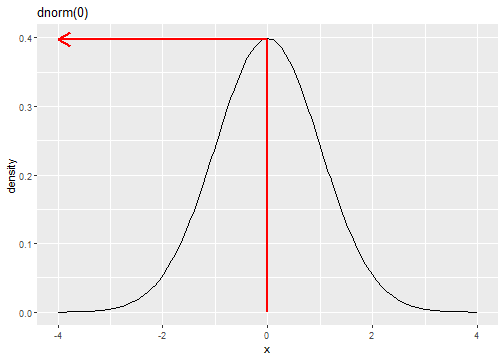 ```r dnorm(0) ``` ``` [1] 0.3989423 ``` --- ## Standard Normal Distribution $$ f_X(x) = \frac{1}{\sqrt{(2\pi)}} e^{-(x)^2/2} $$ ```r pnorm(0) ``` ``` [1] 0.5 ```  --- ## Standard Normal Distribution $$ f_X(x) = \frac{1}{\sqrt{(2\pi)}} e^{-(x)^2/2} $$ ```r pnorm(0) ``` ``` [1] 0.5 ``` 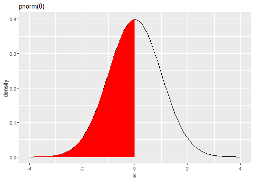 --- ## Standard Normal Distribution $$ f_X(x) = \frac{1}{\sqrt{(2\pi)}} e^{-(x)^2/2} $$ ```r qnorm(0.5) ``` ``` [1] 0 ``` 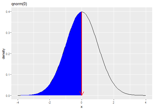 --- ### Standard Normal Distribution: rnorm ```r set.seed(262020) random_numbers <- rnorm(10) random_numbers ``` ``` [1] 0.20078181 0.95873346 1.18369056 1.49513750 1.18109222 -0.57789570 [7] 0.01790671 0.81185245 0.39488199 -0.44337927 ``` ```r sort(random_numbers) ## sort the numbers then it is easy to map with the graph ``` ``` [1] -0.57789570 -0.44337927 0.01790671 0.20078181 0.39488199 0.81185245 [7] 0.95873346 1.18109222 1.18369056 1.49513750 ``` 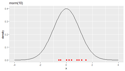<!-- --> --- ## Other distributions in R .pull-left[ - **`beta`**: beta distribution - **`binom`**: binomial distribution - **`cauchy`**: Cauchy distribution - **`chisq`**: chi-squared distribution - **`exp`**: exponential distribution - **`f`**: F distribution - **`gamma`**: gamma distribution - **`geom`**: geometric distribution - **`hyper`**: hyper-geometric distribution ] .pull-right[ - **`lnorm`**: log-normal distribution - **`multinom`**: multinomial distribution - **`nbinom`**: negative binomial distribution - **`norm`**: normal distribution - **`pois`**: Poisson distribution - **`t`**: Student's t distribution - **`unif`**: uniform distribution - **`weibull`**: Weibull distribution ] -- > 🙋 Getting help with R: **`?Distributions`** --- class: duke-orange, center, middle # Your turn --- 1. Suppose `\(Z \sim N(0,1)\)`. Calculate the following standard normal probabilities. - `\(P(Z \le 1.25)\)`, - `\(P(Z > 1.25)\)`, - `\(P(Z \leq -1.25)\)`, - `\(P(-.38 \leq Z \leq 1.25)\)`. 1. Find the following percentiles for the standard normal distribution. - 90th, - 95th, - 97.5th, 1. Determine the `\(Z_\alpha\)` for the following - `\(\alpha = 0.1\)` - `\(\alpha = 0.95\)` --- 1. Suppose `\(X \sim N(15, 9)\)`. Calculate the following probabilities - `\(P(X \leq 15)\)`, - `\(P(X < 15)\)`, - `\(P(X \geq 10)\)`. 1. A particular mobile phone number is used to receive both voice messages and text messages. Suppose 20% of the messages involve text messages, and consider a sample of 15 messages. What is the probability that - At most 8 of the messages involve a text message? - Exactly 8 of the messages involve a text message. 1. Generate 20 random values from a Poisson distribution with mean 10 and calculate the mean. Compare your answer with your friend's answer. --- # Reproducibility of scientific results ```r rnorm(10) # first attempt ``` ``` [1] 1.4701904 -0.2375662 0.1765985 -0.5257483 -1.3674764 -1.4422500 [7] 0.7576607 0.6475122 -1.1543034 0.9066248 ``` ```r rnorm(10) # second attempt ``` ``` [1] -1.7603264 -0.3402939 -1.0335807 1.0645014 -0.3874459 0.5975271 [7] -2.1535707 0.6602928 1.1581404 0.6133446 ``` As you can see above you will get different results ```r set.seed(1) rnorm(10) # First attempt with set.seed ``` ``` [1] -0.6264538 0.1836433 -0.8356286 1.5952808 0.3295078 -0.8204684 [7] 0.4874291 0.7383247 0.5757814 -0.3053884 ``` ```r set.seed(1) rnorm(10) # Second attempt with set.seed ``` ``` [1] -0.6264538 0.1836433 -0.8356286 1.5952808 0.3295078 -0.8204684 [7] 0.4874291 0.7383247 0.5757814 -0.3053884 ``` --- # R Apply family and its variants - **`apply()`** function ```r marks <- data.frame(maths=c(10, 20, 30), chemistry=c(100, NA, 60)) marks ``` ``` maths chemistry 1 10 100 2 20 NA 3 30 60 ``` ```r apply(marks, 1, mean) ``` ``` [1] 55 NA 45 ``` ```r apply(marks, 2, mean) ``` ``` maths chemistry 20 NA ``` -- ```r apply(marks, 1, mean, na.rm=TRUE) ``` ``` [1] 55 20 45 ``` --- class: duke-orange, center, middle # Your turn --- Calculate the row and column wise standard deviation of the following matrix ``` [,1] [,2] [,3] [,4] [1,] 1 6 11 16 [2,] 2 7 12 17 [3,] 3 8 13 18 [4,] 4 9 14 19 [5,] 5 10 15 20 ``` --- class: duke-green, center, middle # Your turn --- ## Assignment 1: Individual Find about the following variants of apply family functions in R **`lapply()`**, **`sapply()`**, **`vapply()`**, **`mapply()`**, **`rapply()`**, and **`tapply()`** functions. Resourses: You can follow the DataCamp tutorial [here](https://www.datacamp.com/community/tutorials/r-tutorial-apply-family?utm_source=adwords_ppc&utm_campaignid=1658343524&utm_adgroupid=63833882055&utm_device=c&utm_keyword=%2Bapply%20%2Br&utm_matchtype=b&utm_network=g&utm_adpostion=&utm_creative=319558765408&utm_targetid=aud-299261629574:kwd-309818754193&utm_loc_interest_ms=&utm_loc_physical_ms=1009919&gclid=EAIaIQobChMImfeQkOTq5wIVVQwrCh1BngrmEAAYASAAEgLEa_D_BwE). - You should clearly explain, - syntax for each function - function inputs - how each function works?/ The task of the function. - output of the function. - differences between the functions (apply vs lapply, apply vs sapply, etc.) - Provide your own example for each function. Use only 1 A4 sheet, you may use both sides. Assignment due date: 3 March 2020 --- ## Data Visualization: qplot() ?qplot --  --- # Installing R Packages ## Method 1 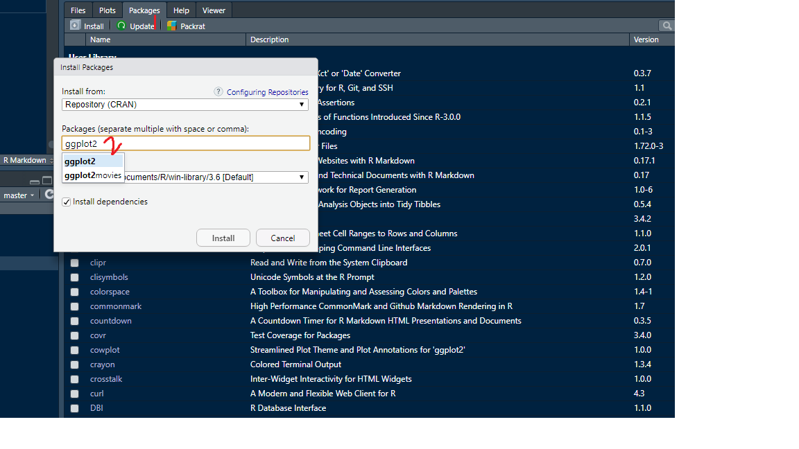 ## Method 2 ```r install.packages("ggplot2") ``` --- ## Load package ```r library(ggplot2) ``` Now search `?qplot` Note: You shouldn't have to re-install packages each time you open R. However, you do need to load the packages you want to use in that session via `library`. --- ## mozzie dataset ```r library(mozzie) data(mozzie) ``` --- ## Data Visualization with `qplot` ## plot vs qplot .pull-left[ ```r plot(mozzie$Colombo, mozzie$Gampaha) ``` <!-- --> ] .pull-right[ ```r qplot(Colombo, Gampaha, data=mozzie) ``` <!-- --> ] --- ## Data Visualization with `qplot` .pull-left[ ```r qplot(Colombo, Gampaha, data=mozzie) ``` <!-- --> ] .pull-right[ ```r qplot(Colombo, Gampaha, data=mozzie, colour=Year) ``` 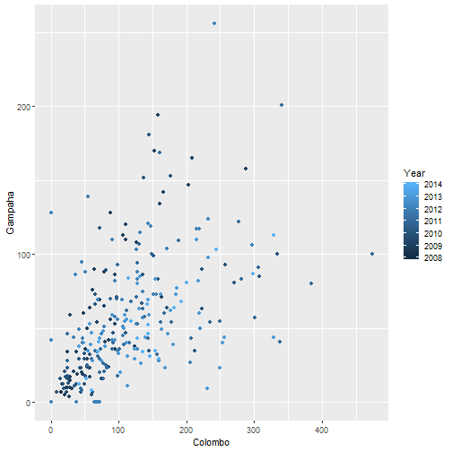<!-- --> ] --- ## Data Visualization with `qplot` .pull-left[ ```r qplot(Colombo, Gampaha, data=mozzie) ``` <!-- --> ] .pull-right[ ```r qplot(Colombo, Gampaha, data=mozzie, size=Year) ``` 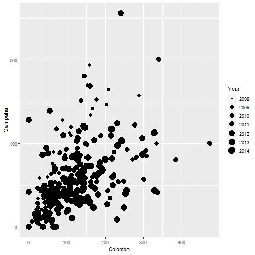<!-- --> ] --- ## Data Visualization with `qplot` .pull-left[ ```r qplot(Colombo, Gampaha, data=mozzie) ``` <!-- --> ] .pull-right[ ```r qplot(Colombo, Gampaha, data=mozzie, geom="point") ``` 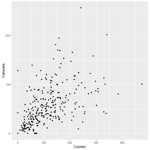<!-- --> ] --- ## Data Visualization with `qplot` .pull-left[ ```r qplot(ID, Gampaha, data=mozzie) ``` <!-- --> ] .pull-right[ ```r qplot(ID, Gampaha, data=mozzie, geom="line") ``` <!-- --> ] --- ## Data Visualization with `qplot` .pull-left[ ```r qplot(ID, Gampaha, data=mozzie) ``` <!-- --> ] .pull-right[ ```r qplot(ID, Gampaha, data=mozzie, geom="path") ``` <!-- --> ] --- ## Data Visualization with `qplot` .pull-left[ ```r qplot(Colombo, Gampaha, data=mozzie, geom="line") ``` <!-- --> ] .pull-right[ ```r qplot(Colombo, Gampaha, data=mozzie, geom="path") ``` <!-- --> ] --- ## Data Visualization with `qplot` .pull-left[ ```r qplot(Colombo, Gampaha, data=mozzie, geom=c("line", "point")) ``` 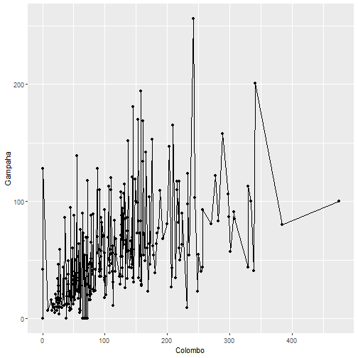<!-- --> ] .pull-right[ ```r qplot(Colombo, Gampaha, data=mozzie, geom=c("path", "point")) ``` 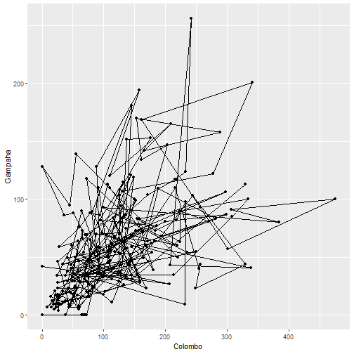<!-- --> ] --- ## Data Visualization with `qplot` .pull-left[ ```r boxplot(Colombo~Year, data=mozzie) ``` 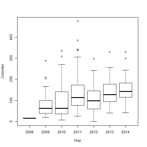<!-- --> ] .pull-right[ ```r qplot(factor(Year), Colombo, data=mozzie, geom="boxplot") ``` 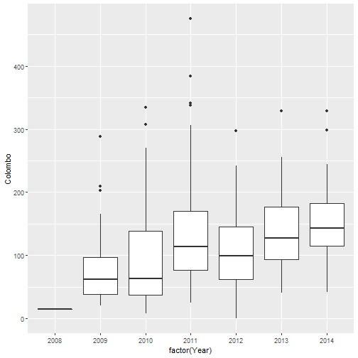<!-- --> ] --- ## Data Visualization with `qplot` .pull-left[ ```r qplot(factor(Year), Colombo, data=mozzie, geom="boxplot") ``` <!-- --> ] .pull-right[ ```r qplot(factor(Year), Colombo, data=mozzie) # geom="point"-default ``` <!-- --> ] --- ## Data Visualization with `qplot` .pull-left[ ```r qplot(factor(Year), Colombo, data=mozzie, geom="point") ``` <!-- --> ] .pull-right[ ```r qplot(factor(Year), Colombo, data=mozzie, geom=c("jitter", "point")) # geom="point"-default ``` <!-- --> ] --- ## Data Visualization with `qplot` .pull-left[ ```r qplot(factor(Year), Colombo, data=mozzie, geom=c("jitter", "point")) ``` <!-- --> ] .pull-right[ ```r qplot(factor(Year), Colombo, data=mozzie, geom=c("jitter", "point", "boxplot")) # geom="point"-default ``` <!-- --> ] --- ## Data Visualization with `qplot` .pull-left[ ```r qplot(Colombo, data=mozzie) ``` ``` `stat_bin()` using `bins = 30`. Pick better value with `binwidth`. ``` <!-- --> ] .pull-right[ ```r qplot(Colombo, data=mozzie, geom="density") ``` <!-- --> ] --- class: duke-orange, center, middle # Your turn --- Explore `iris` dataset with suitable graphics. ```r head(iris) ``` ``` Sepal.Length Sepal.Width Petal.Length Petal.Width Species 1 5.1 3.5 1.4 0.2 setosa 2 4.9 3.0 1.4 0.2 setosa 3 4.7 3.2 1.3 0.2 setosa 4 4.6 3.1 1.5 0.2 setosa 5 5.0 3.6 1.4 0.2 setosa 6 5.4 3.9 1.7 0.4 setosa ``` <img src="iris_flower_dataset.png" width="800"> --- class: center, middle Slides available at: hellor.netlify.com All rights reserved by [Thiyanga S. Talagala](https://thiyanga.netlify.com/)