STA 517 3.0 Programming and Statistical Computing with R🚦Built-in functions in R Dr Thiyanga Talagala1

Function Anatomy

vec1 <- c(1, 2, 3, 4, 5)
mean(vec1)

[1] 3

vec2 <- c(1, 2, NA, 3, 4, 5)
mean(vec2)

[1] NA

Help

?mean

help: `mean`

help: `sort`

`mean` with additional inputs

vec1 <- c(1, 2, 3, 4, 5)
mean(vec1)

[1] 3

vec2 <- c(1, 2, NA, 3, 4, 5)
mean(vec2)

[1] NA

mean(vec2, na.rm=TRUE)

[1] 3

vec <- c(10, 1, 2, 4, 100, 15)
sort(vec)

[1]   1   2   4  10  15 100

sort(vec, decreasing = TRUE)

[1] 100  15  10   4   2   1

sort(vec, decreasing = FALSE)

[1]   1   2   4  10  15 100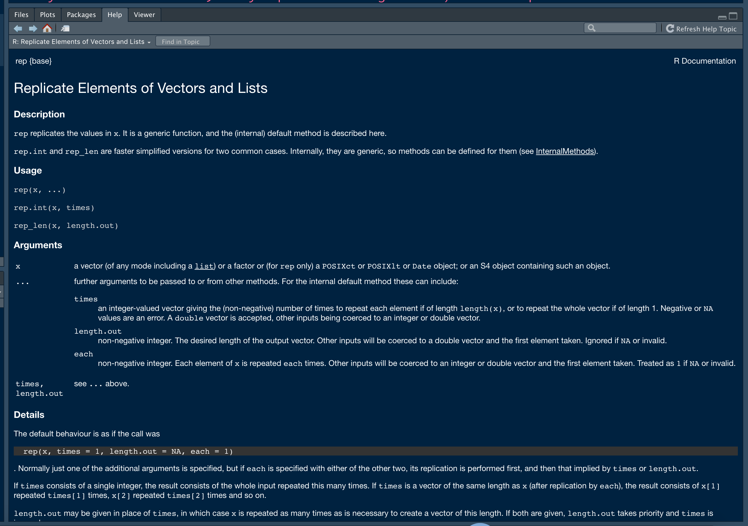

`rep`

Vector creation with `rep` function in R!

Working with built-in functions in R

How to call a built-in function
Arguments matching
Basic functions
Test and type conversion functions
Probability distribution functions
Reproducibility of scientific results
Data visualization: qplot

Functions in R

👉🏻 Perform a specific task according to a set of instructions.

Functions in R

👉🏻 Perform a specific task according to a set of instructions.

👉🏻 Some functions we have discussed so far,

c, matrix, array, list, data.frame, str, dim, length, nrow, which.max, diag, summary

Functions in R

👉🏻 Perform a specific task according to a set of instructions.

👉🏻 Some functions we have discussed so far,

c, matrix, array, list, data.frame, str, dim, length, nrow, which.max, diag, summary

👉🏻 In R, functions are objects of class function.

class(length)

[1] "function"

Functions in R (cont.)

👉🏻 There are basically two types of functions:

💻 Built-in functions

Already created or defined in the programming framework to make our work easier.

👨 User-defined functions

Sometimes we need to create our own functions for a specific purpose.

How to call a built-in function in R

function_name(arg1 = 1, arg2 = 3)

Argument matching

The following calls to mean are all equivalent

mydata <- c(rnorm(20), 100000)
mean(mydata) # matched by position
mean(x = mydata) # matched by name
mean(mydata, na.rm = FALSE)
mean(x = mydata, na.rm = FALSE) 
mean(na.rm = FALSE, x = mydata) 
mean(na.rm = FALSE, mydata)

[1] 4762.105

⚠️ Even though it works, do not change the order of the arguments too much.

Argument matching (cont.)some arguments have default values

mean(mydata, trim=0)

[1] 4762.105
mean(mydata) # Default value for trim is 0

[1] 4762.105
mean(mydata, trim=0.1)

[1] 0.2973882
mean(mydata, tr=0.1) # Partial Matching

[1] 0.2973882
18

?mean19

Your turn20

Calculate the mean of 1, 2, 3, 8, 10, 20, 56, NA.
Arrange the numbers according to the descending order and ascending order.
Compute standard error of the above numbers.

Basic maths functions

Operator	Description

abs(x)	absolute value of x
log(x, base = y)	logarithm of x with base y; if base is not specified, returns the natural logarithm
exp(x)	exponential of x
sqrt(x)	square root of x
factorial(x)	factorial of x

Basic statistic functions

Operator	Description

mean(x)	mean of x
median(x)	median of x
mode(x)	mode of x
var(x)	variance of x
sd(x)	standard deviation of x
scale(x)	z-score of x
quantile(x)	quantiles of x
summary(x)	summary of x: mean, minimum, maximum, etc.

Test and Type conversion functions

Test	Convert

is.numeric()	as.numeric()
is.character()	as.character()
is.vector()	as.vector()
is.matrix()	as.matrix()
is.data.frame()	as.data.frame()
is.factor()	as.factor()
is.logical()	as.logical()
is.na()

Test and Type conversion functions

Test
Convert

is.numeric()
as.numeric()

is.character()
as.character()

is.vector()
as.vector()

is.matrix()
as.matrix()

is.data.frame()
as.data.frame()

is.factor()
as.factor()

is.logical()
as.logical()

is.na()

a <- c(1, 2, 3); a

[1] 1 2 3
is.numeric(a)

[1] TRUE
is.vector(a)

[1] TRUE
25

Test and Type conversion functions

Test	Convert

is.numeric()	as.numeric()
is.character()	as.character()
is.vector()	as.vector()
is.matrix()	as.matrix()
is.data.frame()	as.data.frame()
is.factor()	as.factor()
is.logical()	as.logical()
is.na()

Test and Type conversion functions

Test	Convert

is.numeric()	as.numeric()
is.character()	as.character()
is.vector()	as.vector()
is.matrix()	as.matrix()
is.data.frame()	as.data.frame()
is.factor()	as.factor()
is.logical()	as.logical()
is.na()

b <- as.character(a); b

[1] "1" "2" "3"

is.vector(b)

[1] TRUE

is.character(b)

[1] TRUE

Your turn28

Remove missing values in the following vector

 [1]  0.61940020 -0.93808729  0.95518590 -0.22663938  0.29591186          NA
 [7]  0.36788089  0.71791098  0.71202022  0.22765782          NA          NA
[13] -0.74024324  0.02081516 -0.14979979 -0.22351308  0.98729725          NA
[19]          NA          NA          NA          NA          NA          NA
[25]          NA          NA          NA -1.50016003  0.18682734  0.20808590
[31]  0.70102264 -0.10633074 -1.18460046  0.06475501  0.11568817 -0.04333140
[37] -0.22020064  0.02764713  0.10165760 -0.18234246  1.32914659 -1.29704248
[43]  1.05317749 -0.70109051  0.09798707  0.10457263 -0.21449845

Probability distribution functions

Each probability distribution in R is associated with four functions.
Naming convention for the four functions:

For each function there is a root name. For example, the root name for the normal distribution is norm. This root is prefixed by one of the letters d, p, q, r.
- d prefix for the distribution function
- p prefix for the cumulative probability
- q prefix for the quantile
- r prefix for the random number generator
Example: dnorm, pnorm, qnorm, rnorm

Illustration with Standard normal distribution

The general formula for the probability density function of the normal distribution with mean $μ$ and variance $σ$ is given by

$f_{X} (x) = \frac{1}{σ \sqrt{(2 π)}} e^{- (x - μ)^{2} / 2 σ^{2}}$

If we let the mean $μ = 0$ and the standard deviation $σ = 1$ , we get the probability density function for the standard normal distribution.

$f_{X} (x) = \frac{1}{\sqrt{(2 π)}} e^{- (x)^{2} / 2}$

Standard Normal Distribution

$f_{X} (x) = \frac{1}{\sqrt{(2 π)}} e^{- (x)^{2} / 2}$

dnorm(0)

[1] 0.3989423

Standard normal probability density function: dnorm(0)

Standard Normal Distribution

$f_{X} (x) = \frac{1}{\sqrt{(2 π)}} e^{- (x)^{2} / 2}$

pnorm(0)

[1] 0.5

Standard normal probability density function: pnorm(0)

Standard Normal Distribution

$f_{X} (x) = \frac{1}{\sqrt{(2 π)}} e^{- (x)^{2} / 2}$

qnorm(0.5)

[1] 0

Standard normal probability density function: qnorm(0.5)

Normal distribution: `norm`

pnorm(3)

[1] 0.9986501

pnorm(3, sd=1, mean=0)

[1] 0.9986501

pnorm(3, sd=2, mean=1)

[1] 0.8413447

Binomial distribution

dbinom(2, size=10, prob=0.2)

[1] 0.3019899

a <- dbinom(0:10, size=10, prob=0.2)
a

 [1] 0.1073741824 0.2684354560 0.3019898880 0.2013265920 0.0880803840
 [6] 0.0264241152 0.0055050240 0.0007864320 0.0000737280 0.0000040960
[11] 0.0000001024

cumsum(a)

 [1] 0.1073742 0.3758096 0.6777995 0.8791261 0.9672065 0.9936306 0.9991356
 [8] 0.9999221 0.9999958 0.9999999 1.0000000

cumsum(a)

 [1] 0.1073742 0.3758096 0.6777995 0.8791261 0.9672065 0.9936306 0.9991356
 [8] 0.9999221 0.9999958 0.9999999 1.0000000

pbinom(0:10, size=10, prob=0.2)

 [1] 0.1073742 0.3758096 0.6777995 0.8791261 0.9672065 0.9936306 0.9991356
 [8] 0.9999221 0.9999958 0.9999999 1.0000000

qbinom(0.4, size=10, prob=0.2)

[1] 2

Standard Normal Distribution: rnorm

set.seed(262020)
random_numbers <- rnorm(5)
random_numbers

[1] 0.2007818 0.9587335 1.1836906 1.4951375 1.1810922

sort(random_numbers) ## sort the numbers then it is easy to map with the graph

[1] 0.2007818 0.9587335 1.1810922 1.1836906 1.4951375

Other distributions in R40

beta: beta distribution
binom: binomial distribution
cauchy: Cauchy distribution
chisq: chi-squared distribution
exp: exponential distribution
f: F distribution
gamma: gamma distribution
geom: geometric distribution
hyper: hyper-geometric distribution

lnorm: log-normal distribution
multinom: multinomial distribution
nbinom: negative binomial distribution
norm: normal distribution
pois: Poisson distribution
t: Student's t distribution
unif: uniform distribution
weibull: Weibull distribution

🙋 Getting help with R: ?Distributions

Your turn43

Q1 Suppose $Z \sim N (0, 1)$ . Calculate the following standard normal probabilities.

$P (Z \leq 1.25)$ ,
$P (Z > 1.25)$ ,
$P (Z \leq - 1.25)$ ,
$P (- .38 \leq Z \leq 1.25)$ .

Q2 Find the following percentiles for the standard normal distribution.

90th,
95th,
97.5th,

Q3 Determine the $Z_{α}$ for the following

$α = 0.1$
$α = 0.95$

Q4 Suppose $X \sim N (15, 9)$ . Calculate the following probabilities

$P (X \leq 15)$ ,
$P (X < 15)$ ,
$P (X \geq 10)$ .

02:00

Q5 A particular mobile phone number is used to receive both voice messages and text messages. Suppose 20% of the messages involve text messages, and consider a sample of 15 messages. What is the probability that

At most 8 of the messages involve a text message?
Exactly 8 of the messages involve a text message.

02:00

Q6 Generate 20 random values from a Poisson distribution with mean 10 and calculate the mean. Compare your answer with others.

02:00

Reproducibility of scientific results

rnorm(10) # first attempt

 [1]  1.6582609 -1.8912734 -2.8471112 -2.1617741  0.6401224 -0.4295948
 [7] -0.3122580 -1.0267992  1.4231150  0.8661058

rnorm(10) # second attempt

 [1] -0.91879540 -0.06053766 -0.20263170 -0.26301690  0.97964620 -0.46034817
 [7]  0.81826880 -0.60935778  1.71086661  0.49294451

As you can see above you will get different results.

Reproducibility of scientific results (cont.)

set.seed(1)
rnorm(10) # First attempt with set.seed

 [1] -0.6264538  0.1836433 -0.8356286  1.5952808  0.3295078 -0.8204684
 [7]  0.4874291  0.7383247  0.5757814 -0.3053884

set.seed(1)
rnorm(10) # Second attempt with set.seed

 [1] -0.6264538  0.1836433 -0.8356286  1.5952808  0.3295078 -0.8204684
 [7]  0.4874291  0.7383247  0.5757814 -0.3053884

R Apply family and its variants

apply() function

marks <- data.frame(maths=c(10, 20, 30), chemistry=c(100, NA, 60)); marks

  maths chemistry
1    10       100
2    20        NA
3    30        60

apply(marks, 1, mean)

[1] 55 NA 45

apply(marks, 2, mean)

    maths chemistry 
       20        NA

apply(marks, 1, mean, na.rm=TRUE)

[1] 55 20 45

Your turn52

Calculate the row and column wise standard deviation of the following matrix

     [,1] [,2] [,3] [,4]
[1,]    1    6   11   16
[2,]    2    7   12   17
[3,]    3    8   13   18
[4,]    4    9   14   19
[5,]    5   10   15   20

03:00

Your turn54

Your turn

Find about the following variants of apply family functions in R lapply(), sapply(), vapply(), mapply(), rapply(), and tapply() functions.

Resourses: You can follow the DataCamp tutorial here.

You should clearly explain,
- syntax for each function/ Provide your own example for each function
- function inputs
- how each function works?/ The task of the function.
- output of the function.
- differences between the functions (apply vs lapply, apply vs sapply, etc.)

Data Visualization: qplot()

?qplot

Data Visualization: qplot()

?qplot

Installing R Packages

Method 1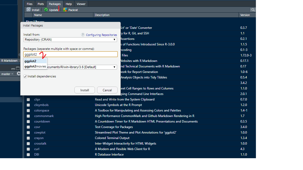

Installing R Packages

Method 2

install.packages("ggplot2")

Load package

library(ggplot2)

Now search ?qplot

Note: You shouldn't have to re-install packages each time you open R. However, you do need to load the packages you want to use in that session via library.

`install.packages` vs `library`

Image credit: Professor Di Cook

mozzie dataset

library(mozzie)
data(mozzie)

Data Visualization with R

boxplot(mpg ~ cyl, data = mtcars,   
        xlab = "Quantity of Cylinders",  
        ylab = "Miles Per Gallon",   
        main = "Boxplot Example",  
        notch = TRUE,   
        varwidth = TRUE,   
        col = c("green","yellow","red"),  
        names = c("High","Medium","Low")  
)

counts <- table(mtcars$gear)
barplot(counts, main="Car Distribution",
   xlab="Number of Gears")

Default R installation: graphics package

 [1] "abline"          "arrows"          "assocplot"       "axis"           
 [5] "Axis"            "axis.Date"       "axis.POSIXct"    "axTicks"        
 [9] "barplot"         "barplot.default" "box"             "boxplot"        
[13] "boxplot.default" "boxplot.matrix"  "bxp"             "cdplot"         
[17] "clip"            "close.screen"    "co.intervals"    "contour"        
[21] "contour.default" "coplot"          "curve"           "dotchart"       
[25] "erase.screen"    "filled.contour"  "fourfoldplot"    "frame"          
[29] "grconvertX"      "grconvertY"      "grid"            "hist"           
[33] "hist.default"    "identify"        "image"           "image.default"  
[37] "layout"          "layout.show"     "lcm"             "legend"         
[41] "lines"           "lines.default"   "locator"         "matlines"       
[45] "matplot"         "matpoints"       "mosaicplot"      "mtext"          
[49] "pairs"           "pairs.default"   "panel.smooth"    "par"            
[53] "persp"           "pie"             "plot"            "plot.default"   
[57] "plot.design"     "plot.function"   "plot.new"        "plot.window"    
[61] "plot.xy"         "points"          "points.default"  "polygon"        
[65] "polypath"        "rasterImage"     "rect"            "rug"            
[69] "screen"          "segments"        "smoothScatter"   "spineplot"      
[73] "split.screen"    "stars"           "stem"            "strheight"      
[77] "stripchart"      "strwidth"        "sunflowerplot"   "symbols"        
[81] "text"            "text.default"    "title"           "xinch"          
[85] "xspline"         "xyinch"          "yinch"

mozzie

head(mozzie)

# A tibble: 6 × 28
     ID  Year  Week Colombo Gampaha Kalutara Kandy Matale `Nuwara Eliya` Galle
  <int> <int> <int>   <int>   <int>    <int> <int>  <int>          <int> <int>
1     1  2008    52      15       7        1    11      4              0     0
2     2  2009     1      44      23        5    16     21              2     0
3     3  2009     2      39      19       11    42      9              1     2
4     4  2009     3      57      23       12    28      3              2     1
5     5  2009     4      53      24       19    32     20              2     2
6     6  2009     5      29      17       10    21      6              0     3
# … with 18 more variables: Hambantota <int>, Matara <int>, Jaffna <int>,
#   Kilinochchi <int>, Mannar <int>, Vavuniya <int>, Mulative <int>,
#   Batticalo <int>, Ampara <int>, Trincomalee <int>, Kurunagala <int>,
#   Puttalam <int>, Anuradhapura <int>, Polonnaruwa <int>, Badulla <int>,
#   Monaragala <int>, Ratnapura <int>, Kegalle <int>

Data Visualization with `qplot`

plot vs qplot

plot(mozzie$Colombo, mozzie$Gampaha)

qplot(Colombo, Gampaha, data=mozzie)

Data Visualization with `qplot`

qplot(Colombo, Gampaha, data=mozzie)

qplot(Colombo, Gampaha, data=mozzie,
      colour=Year)

Data Visualization with `qplot`

qplot(Colombo, Gampaha, data=mozzie)

qplot(Colombo, Gampaha, data=mozzie, 
      size=Year)

Data Visualization with `qplot`

qplot(Colombo, Gampaha, data=mozzie)

qplot(Colombo, Gampaha, data=mozzie, 
      size=Year, alpha=0.5)

Data Visualization with `qplot`

qplot(Colombo, Gampaha, data=mozzie)

qplot(Colombo, Gampaha, data=mozzie,
      geom="point")

Data Visualization with `qplot`

qplot(ID, Gampaha, data=mozzie)

qplot(ID, Gampaha, data=mozzie, 
      geom="line")

Data Visualization with `qplot`

qplot(ID, Gampaha, data=mozzie)

qplot(ID, Gampaha, data=mozzie,
      geom="path")

Data Visualization with `qplot`

qplot(Colombo, Gampaha, data=mozzie,
      geom="line")

qplot(Colombo, Gampaha, data=mozzie, 
      geom="path")

Data Visualization with `qplot`

qplot(Colombo, Gampaha, data=mozzie, 
      geom=c("line", "point"))

qplot(Colombo, Gampaha, data=mozzie,
      geom=c("path", "point"))

Data Visualization with `qplot`

boxplot(Colombo~Year, data=mozzie)

qplot(factor(Year), Colombo, data=mozzie,
      geom="boxplot")

Data Visualization with `qplot`

qplot(factor(Year), Colombo, data=mozzie,
      geom="boxplot")

qplot(factor(Year), Colombo, data=mozzie) # geom="point"-default

Data Visualization with `qplot`

qplot(factor(Year), Colombo, data=mozzie, 
      geom="point")

qplot(factor(Year), Colombo, data=mozzie, 
      geom="jitter") # geom="point"-default

Data Visualization with `qplot`

qplot(factor(Year), Colombo, data=mozzie,
      geom="jitter")

qplot(factor(Year), Colombo, data=mozzie,
      geom=c("jitter", "boxplot")) # geom="point"-default

qplot(factor(Year), Colombo, data=mozzie,
      geom=c("jitter", "boxplot")) # geom="point"-default

qplot(factor(Year), Colombo, data=mozzie,
      geom=c("jitter", "boxplot")) # geom="point"-default

qplot(factor(Year), Colombo, data=mozzie,
      geom=c("jitter", "boxplot"),
      outlier.shape = NA) # geom="point"-default

Data Visualization with `qplot`

qplot(Colombo, data=mozzie)

qplot(Colombo, data=mozzie, geom="density")

Your turn85

Explore iris dataset with suitable graphics.

head(iris)

  Sepal.Length Sepal.Width Petal.Length Petal.Width Species
1          5.1         3.5          1.4         0.2  setosa
2          4.9         3.0          1.4         0.2  setosa
3          4.7         3.2          1.3         0.2  setosa
4          4.6         3.1          1.5         0.2  setosa
5          5.0         3.6          1.4         0.2  setosa
6          5.4         3.9          1.7         0.4  setosa

↑, ←, Pg Up, k	Go to previous slide
↓, →, Pg Dn, Space, j	Go to next slide
Home	Go to first slide
End	Go to last slide
Number + Return	Go to specific slide
b / m / f	Toggle blackout / mirrored / fullscreen mode
c	Clone slideshow
p	Toggle presenter mode
t	Restart the presentation timer
?, h	Toggle this help

STA 517 3.0 Programming and Statistical Computing with R

🚦Built-in functions in R

Dr Thiyanga Talagala

Function Anatomy

Help

help: mean

help: sort

mean with additional inputs

rep

Vector creation with rep function in R!

Working with built-in functions in R

Functions in R

Functions in R

Functions in R

Functions in R (cont.)

How to call a built-in function in R

Argument matching (cont.)

?mean

Your turn

Basic maths functions

Basic statistic functions

Test and Type conversion functions

Test and Type conversion functions

Test and Type conversion functions

Test and Type conversion functions

Your turn

Probability distribution functions

Illustration with Standard normal distribution

Standard Normal Distribution

Standard Normal Distribution

Standard Normal Distribution

Normal distribution: norm

Binomial distribution

Standard Normal Distribution: rnorm

Other distributions in R

Your turn

Reproducibility of scientific results

Reproducibility of scientific results (cont.)

R Apply family and its variants

Your turn

Your turn

Data Visualization: qplot()

Data Visualization: qplot()

Installing R Packages

Method 1

Installing R Packages

Method 2

Load package

install.packages vs library

mozzie dataset

Data Visualization with R

mozzie

Data Visualization with qplot

plot vs qplot

Data Visualization with qplot

Data Visualization with qplot

Data Visualization with qplot

Data Visualization with qplot

Data Visualization with qplot

Data Visualization with qplot

Data Visualization with qplot

Data Visualization with qplot

Data Visualization with qplot

Data Visualization with qplot

Data Visualization with qplot

Data Visualization with qplot

Data Visualization with qplot

Your turn

Thank you!

Function Anatomy

Help

Help

help: `mean`

help: `sort`

`mean` with additional inputs

`rep`

Vector creation with `rep` function in R!

Normal distribution: `norm`

`install.packages` vs `library`

Data Visualization with `qplot`

Data Visualization with `qplot`

Data Visualization with `qplot`

Data Visualization with `qplot`

Data Visualization with `qplot`

Data Visualization with `qplot`

Data Visualization with `qplot`

Data Visualization with `qplot`

Data Visualization with `qplot`

Data Visualization with `qplot`

Data Visualization with `qplot`

Data Visualization with `qplot`

Data Visualization with `qplot`

Data Visualization with `qplot`